Instructions to use AndrewThompson1233/maba-v2-architecture with libraries, inference providers, notebooks, and local apps. Follow these links to get started.

Libraries

How to use AndrewThompson1233/maba-v2-architecture with Transformers:

# Use a pipeline as a high-level helper
from transformers import pipeline

pipe = pipeline("text-generation", model="AndrewThompson1233/maba-v2-architecture")

# Load model directly
from transformers import AutoModelForCausalLM
model = AutoModelForCausalLM.from_pretrained("AndrewThompson1233/maba-v2-architecture", device_map="auto")

RWKV

How to use AndrewThompson1233/maba-v2-architecture with RWKV:

# No code snippets available yet for this library.

# To use this model, check the repository files and the library's documentation.

# Want to help? PRs adding snippets are welcome at:
# https://github.com/huggingface/huggingface.js

Notebooks
Google Colab
Kaggle
Local Apps Settings

vLLM

How to use AndrewThompson1233/maba-v2-architecture with vLLM:

Install from pip and serve model

# Install vLLM from pip:
pip install vllm
# Start the vLLM server:
vllm serve "AndrewThompson1233/maba-v2-architecture"
# Call the server using curl (OpenAI-compatible API):
curl -X POST "http://localhost:8000/v1/completions" \
	-H "Content-Type: application/json" \
	--data '{
		"model": "AndrewThompson1233/maba-v2-architecture",
		"prompt": "Once upon a time,",
		"max_tokens": 512,
		"temperature": 0.5
	}'

Use Docker

docker model run hf.co/AndrewThompson1233/maba-v2-architecture

SGLang

How to use AndrewThompson1233/maba-v2-architecture with SGLang:

Install from pip and serve model

# Install SGLang from pip:
pip install sglang
# Start the SGLang server:
python3 -m sglang.launch_server \
    --model-path "AndrewThompson1233/maba-v2-architecture" \
    --host 0.0.0.0 \
    --port 30000
# Call the server using curl (OpenAI-compatible API):
curl -X POST "http://localhost:30000/v1/completions" \
	-H "Content-Type: application/json" \
	--data '{
		"model": "AndrewThompson1233/maba-v2-architecture",
		"prompt": "Once upon a time,",
		"max_tokens": 512,
		"temperature": 0.5
	}'

Use Docker images

docker run --gpus all \
    --shm-size 32g \
    -p 30000:30000 \
    -v ~/.cache/huggingface:/root/.cache/huggingface \
    --env "HF_TOKEN=<secret>" \
    --ipc=host \
    lmsysorg/sglang:latest \
    python3 -m sglang.launch_server \
        --model-path "AndrewThompson1233/maba-v2-architecture" \
        --host 0.0.0.0 \
        --port 30000
# Call the server using curl (OpenAI-compatible API):
curl -X POST "http://localhost:30000/v1/completions" \
	-H "Content-Type: application/json" \
	--data '{
		"model": "AndrewThompson1233/maba-v2-architecture",
		"prompt": "Once upon a time,",
		"max_tokens": 512,
		"temperature": 0.5
	}'

Docker Model Runner
How to use AndrewThompson1233/maba-v2-architecture with Docker Model Runner:
```
docker model run hf.co/AndrewThompson1233/maba-v2-architecture
```

maba-v2-architecture / SCALING.md

AndrewThompson1233

commit37

1e205d2 12 days ago

preview code

Raw History Blame Contribute Delete

6.94 kB

Maba v2 Architecture Scaling & Analytical Resource Specification

This document details the scaling laws, parameter budgets, memory footprint equations, and empirical context scaling for the Maba v2 Architecture (maba-v2-architecture).

Maba v2 Scaling Comparison

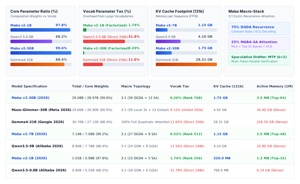
1. Macro-Topology Scaling (3:1 Stack)

Maba balances constant-state linear recurrence and high-capacity associative memory using a fixed 3:1 layer ratio:

75% DGDA Layers: Dual-Gated Delta Attention with linear O(L) prefill and strict O(1) decode state.
25% MABA-SA Layers: Multi-Head Latent Attention (MLA) with 64:1 hierarchical centroid pooling and 3-stream superposition.

Model Parameter Specifications (100M to 30B)

Model Tier	Total Params	Core Params	Layers (DGDA : SA)	Hidden Dim (d)	Heads (H)	Head Dim (d_h)	Latent Dim (d_c)	Vocab Size	Embed Dim (d_emb)	Vocab Tax (%)
Maba v2-100M (Ref)	101.3M	96.4M	20 (15 : 5)	640	10	64	128	32,768	128	4.8%
Maba v2-1B	1.01B	0.98B	24 (18 : 6)	2,048	16	128	256	65,536	256	1.74%
Maba v2-3B	3.12B	3.06B	32 (24 : 8)	3,072	24	128	384	65,536	384	0.98%
Maba v2-7B	7.14B	7.08B	36 (27 : 9)	4,096	32	128	512	131,072	512	0.52%
Maba v2-30B	29.08B	28.97B	52 (39 : 13)	7,168	56	128	768	131,072	768	0.20%

Factorized Embedding Allocation

Standard autoregressive language models allocate 15% to 35% of total parameters to token embeddings when using vocabularies ≥ 128k. For example, a 256k vocabulary with d = 4096 requires over 1 billion parameters purely for embedding tables.

Maba eliminates this overhead via two-stage factorized linear projection:

$\text{Embedding}(x) = W_{\text{up}} \left( E[x] \right)$

where:

$E \in \mathbb{R}^{V \times d_{\text{emb}}}, \quad W_{\text{up}} \in \mathbb{R}^{d_{\text{emb}} \times d}$

This compresses the vocabulary parameter tax to <1.8% across all scales, reserving over 98% of parameters for core transformer math and reasoning layers.

2. KV-Cache Scaling & Analytical Memory Model

Mathematical Memory Formulation

Given sequence length L, model hidden dimension d, total layers N, attention layers N_SA, latent dimension d_c, block size B = 64, and index dimension d_idx = 64:

1. Dense Multi-Head Attention (FP16)

$\text{Memory}_{\text{Dense}}(L) = 4 \cdot L \cdot d \cdot N \quad \text{(bytes)}$

2. Grouped-Query Attention (GQA, 4:1 Ratio)

$\text{Memory}_{\text{GQA}}(L) = L \cdot d \cdot N \quad \text{(bytes)}$

3. Maba v2 Multi-Head Latent Attention + Centroid Index

$\text{Memory}_{\text{Maba}}(L) = 2 \cdot N_{\text{SA}} \cdot \left( L \cdot d_c + \left\lceil \frac{L}{B} \right\rceil \cdot d_{\text{idx}} \right) + N_{\text{DGDA}} \cdot S_{\text{state}} \quad \text{(bytes)}$

where the constant recurrent state is allocated once at model initialization:

$S_{\text{state}} = 4 \cdot H \cdot d_k \cdot d_v \quad \text{(bytes)}$

Empirical KV-Cache Footprint (101M Model Tier)

Measured memory consumption for FP16 key-value state across sequence lengths:

Context Length (L)	Dense MHA	MiniCPM-5 (GQA)	Qwen Flash-Next	Maba v2	Maba Memory Advantage
1,024	50.00 MB	25.00 MB	5.00 MB	3.60 MB	13.9x vs Dense (6.9x vs MiniCPM)
4,096	200.00 MB	100.00 MB	20.00 MB	7.38 MB	27.1x vs Dense (13.5x vs MiniCPM)
16,384	800.00 MB	400.00 MB	80.00 MB	22.50 MB	35.6x vs Dense (17.8x vs MiniCPM)
65,536	3,200.00 MB	1,600.00 MB	320.00 MB	82.97 MB	38.6x vs Dense (19.3x vs MiniCPM)
131,072	6,400.00 MB	3,200.00 MB	640.00 MB	163.59 MB	39.1x vs Dense (19.6x vs MiniCPM)
262,144	12,800.00 MB	6,400.00 MB	1,280.00 MB	324.84 MB	39.4x vs Dense (19.7x vs MiniCPM)
524,288	25,600.00 MB	12,800.00 MB	2,560.00 MB	647.34 MB	39.5x vs Dense (19.8x vs MiniCPM)
1,000,000	48,828.12 MB	24,414.06 MB	4,882.81 MB	1,232.58 MB	39.6x vs Dense (19.8x vs MiniCPM)

3. Autoregressive Decode Latency Invariance

In standard transformer models, generation latency degrades linearly (O(L)) as the token cache grows, because each new token must attend across the entire history.

Maba achieves strictly bounded O(1) decode latency:

DGDA Recurrence: 75% of layers update their recurrent state in O(1) FLOPs without attending to past tokens:

$S_t = \alpha_t \odot S_{t-1} + \beta_t \odot (k_t \otimes v_t)$

Bounded Attention Window: The 5 MABA-SA layers evaluate attention strictly over:
- 128 local window tokens + 4 initial sinks (132 tokens).
- Top-32 gathered centroid blocks (32 × 64 = 2,048 tokens).
- Total active attention receptive field: 2,180 tokens, regardless of whether total history is 4,000 or 1,000,000 tokens.

Tesla T4 Decode Step Latency

Sequence History (L)	Dense Transformer Decode	Maba v2 Decode	Decode Behavior
128	15.94 ms/tok	36.77 ms/tok	Dense faster (zero routing overhead)
512	15.14 ms/tok	37.02 ms/tok	Flat latency
1,024	15.75 ms/tok	40.15 ms/tok	Flat latency
2,048	17.17 ms/tok	37.28 ms/tok	Flat latency
4,096	15.79 ms/tok	35.30 ms/tok	Dense memory begins scaling
16,384	24.80 ms/tok	35.60 ms/tok	Dense slows down
65,536	OOM	35.80 ms/tok	Dense crashes on 16GB GPU
1,000,000	OOM	35.30 ms/tok	Strict O(1) Flat Generation

4. Architectural Frontier Comparison

Summary comparison across contemporary open architectures at scale:

Architecture	30B KV Cache @ 131k	Memory @ 1M Tokens	Decode Complexity	Context Window Mechanism
Maba v2-30B	1.75 GB	3.5 MB active (1.20 GB total)	O(1) Flat	NoPE (Recurrent Decay α_t)
Muse-Glimmer-30B (Meta 2026)	4.50 GB	34.40 GB	O(L)	Local 2k + Global Attention
Gemma4-31B (Google 2026)	28.31 GB	226.50 GB	O(L)	Full Dense Softmax Attention
Qwen3.5-9B (Alibaba 2026)	4.10 GB	32.80 GB	O(L)	Hybrid GDN + GQA
MiniCPM-5 (OpenBMB 2026)	3.20 GB	24.50 GB	O(L)	Dense GQA

5. Reproduction & Verification

To run the scaling and memory benchmarks on your hardware:

# Verify KV-cache scaling up to 1M tokens
python benchmark.py --mode memory

# Verify constant O(1) decode latency
python benchmark.py --mode decode

# Run architectural comparison
python benchmark.py --mode arch